Price Determination
Equilibrium Price and Quantity
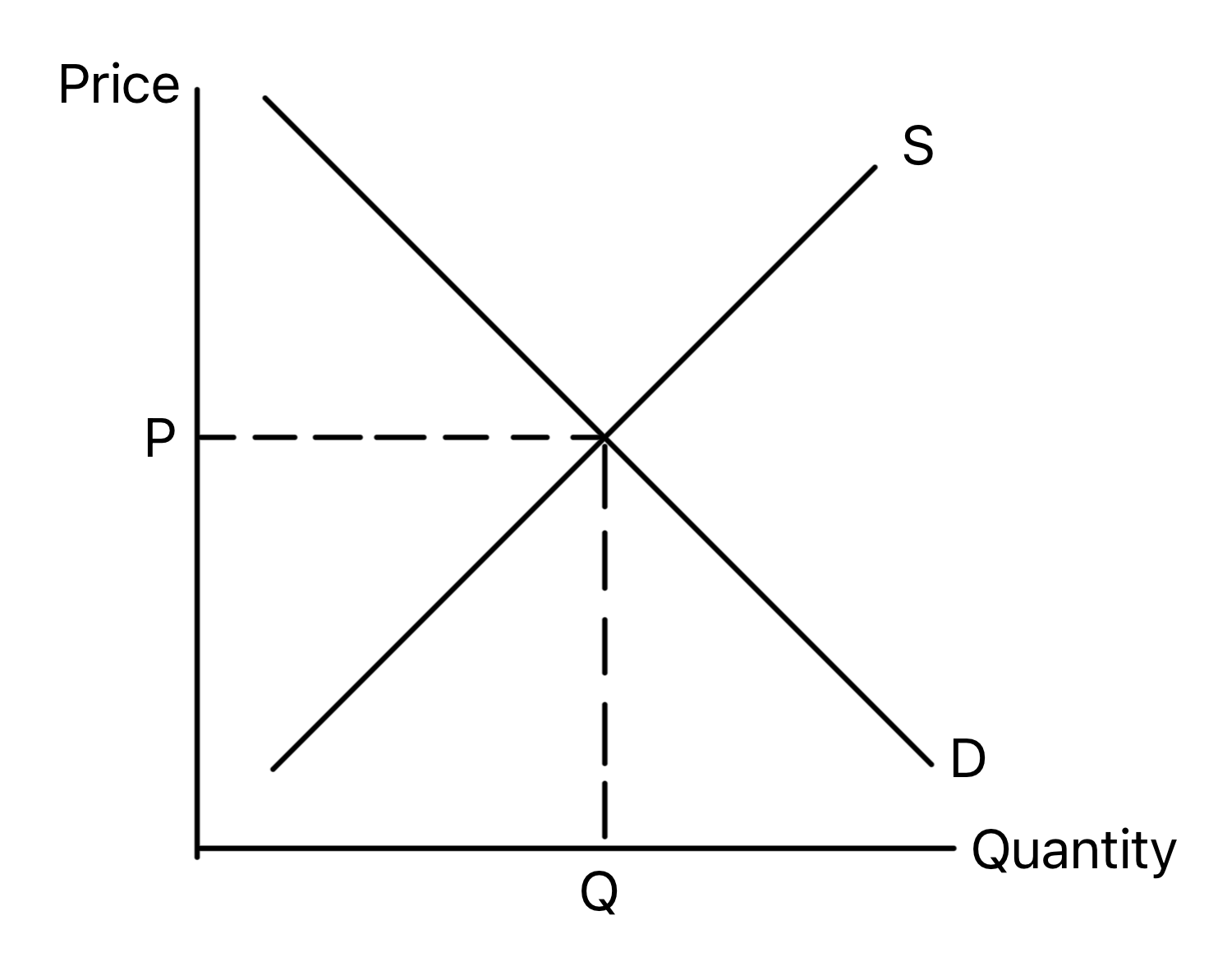
Put the demand curve from 1.3.1 and the supply curve from 1.3.2 on the same diagram and they cross at one point.
Equilibrium price: the price at which the quantity consumers want to buy equals the quantity producers want to sell. It is also called the market-clearing price, because nothing is left unsold and no buyer who will pay that price goes without.
The equilibrium quantity is the amount bought and sold at that price. Once a market reaches equilibrium, there is no pressure for the price to change.
Excess Demand and Excess Supply
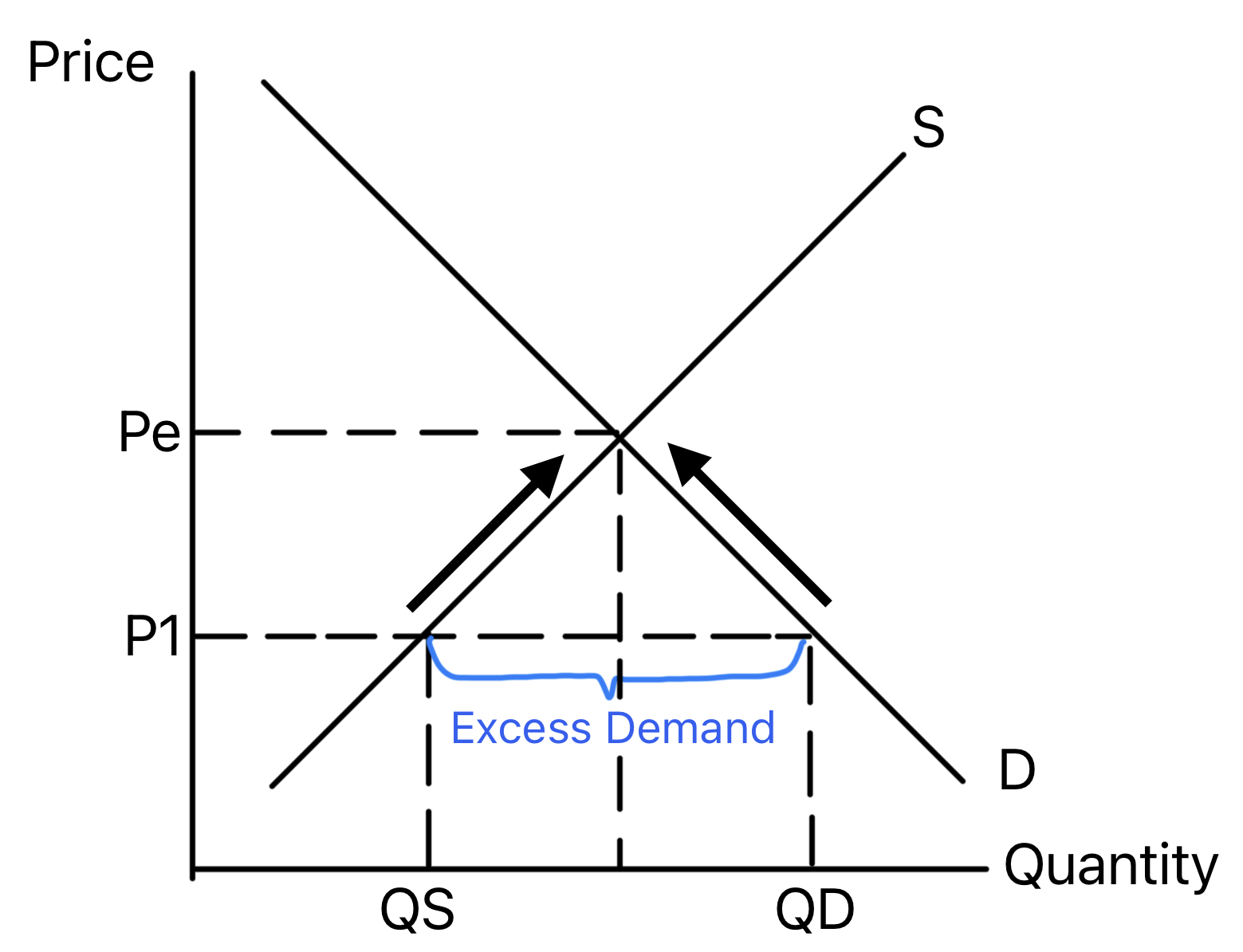
Excess demand: when the quantity demanded is greater than the quantity supplied, because the price is below equilibrium. It shows up as a shortage.
Excess supply: when the quantity supplied is greater than the quantity demanded, because the price is above equilibrium. It shows up as a surplus.
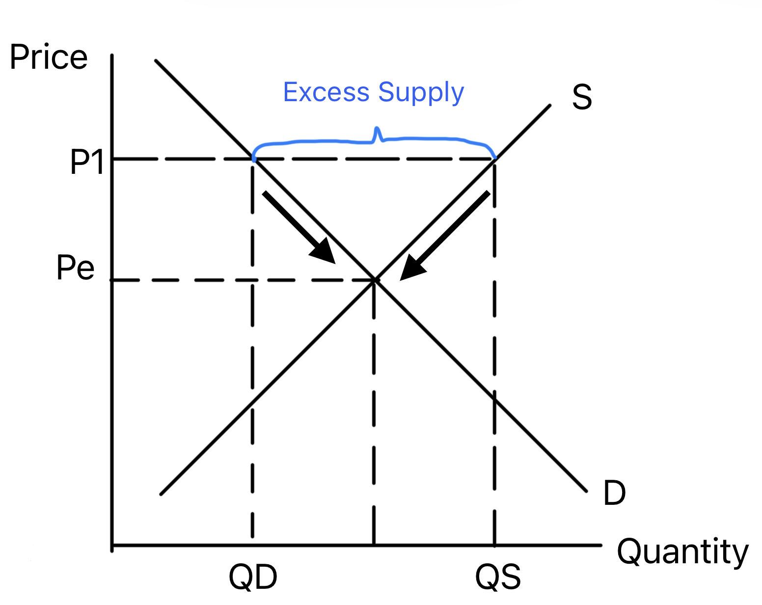
On both diagrams the excess is the horizontal distance between the two curves at P1. Label it, and mark QD and QS on the quantity axis.
How Market Forces Remove Excess Demand and Supply
Excess demand pushes the price up. Shops sell out and queues form, so buyers are prepared to pay more and sellers see they can charge more. As the price rises, demand contracts and supply extends. That carries on until the two are equal again at Pe (the arrows in Figure 2).
Excess supply pushes the price down. Sellers are left with unsold stock, so they cut prices to clear it. As the price falls, demand extends and supply contracts until the market clears at Pe (the arrows in Figure 3).
Using Supply and Demand in Real-World Situations
A shift in demand or supply leaves a shortage or surplus at the old price, and market forces then move the price to a new equilibrium.
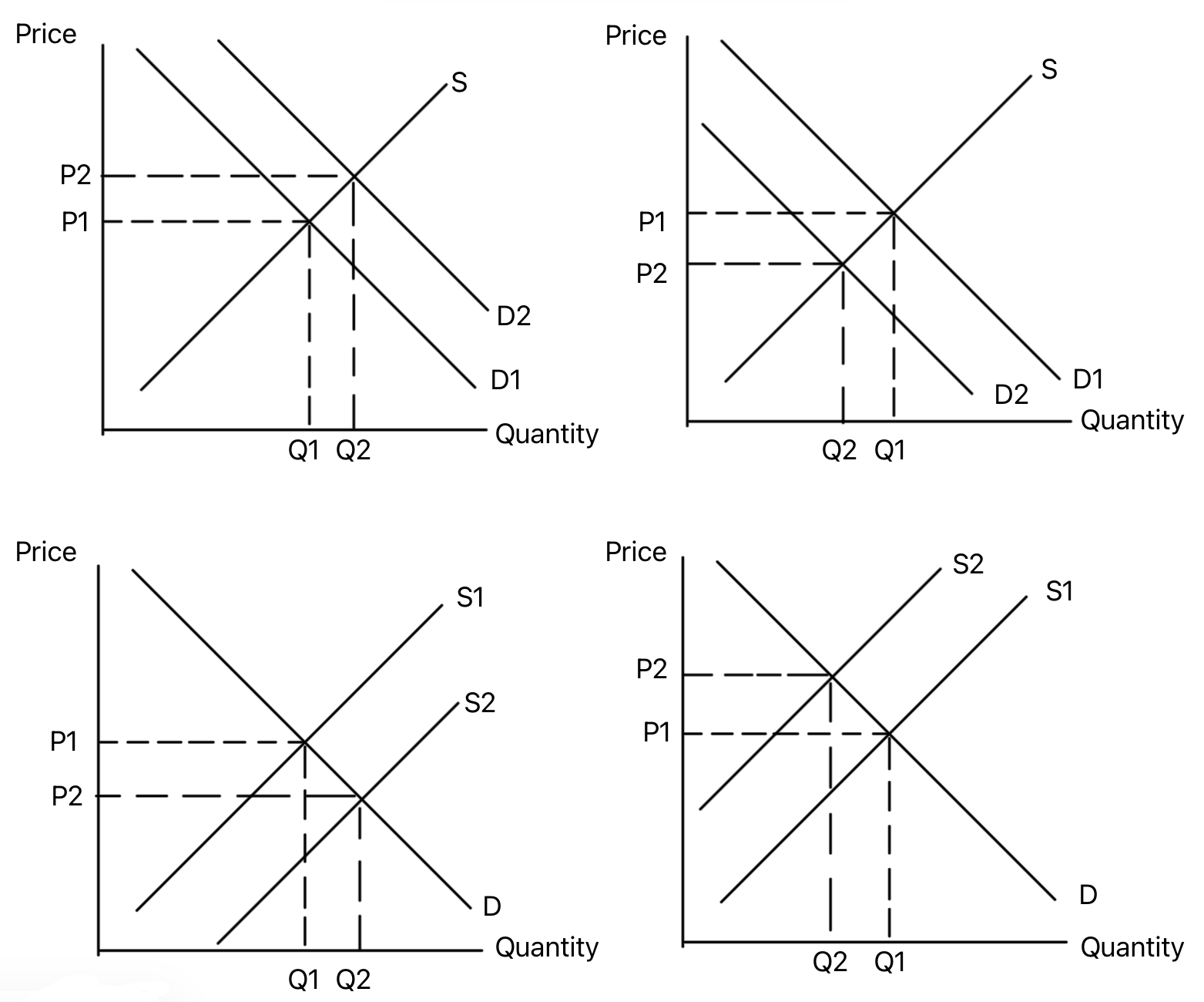
| Change | At the old price | New P and Q | Example |
|---|---|---|---|
| Demand shifts right | Excess demand, so the price rises | P up, Q up | A heatwave and electric fans |
| Demand shifts left | Excess supply, so the price falls | P down, Q down | Winter coats after a mild winter |
| Supply shifts right | Excess supply, so the price falls | P down, Q up | A bumper strawberry harvest |
| Supply shifts left | Excess demand, so the price rises | P up, Q down | The poor cocoa harvests of 2023/24 (see 1.3.2) |
In an exam answer, work through the same steps each time: name the factor, say which curve shifts and which way, explain the shortage or surplus at the old price, then state the new price and quantity.
Limitations of the Supply and Demand Model
Real markets often behave differently from the model:
- Ceteris paribus rarely holds. In the real world several factors change at once. If demand and supply both rise, quantity goes up, but the price could go either way depending on which shift is bigger.
- Time lags. Supply often cannot respond quickly. A farmer cannot grow more wheat until the next harvest, and new houses take years to plan and build, so shortages can last.
- Imperfect information. Buyers and sellers do not know where the equilibrium is. They find it by trial and error. People also buy out of habit or on impulse, which the model leaves out.
- Non-price factors. Many firms compete on quality, brand and service, and change prices only now and then. Contracts and printed price lists slow price changes down.
- Markets that do not clear. Some prices are held away from equilibrium on purpose. Tickets for big concerts are often priced below what fans would pay, so excess demand remains and tickets sell out within minutes.
Use the limits to evaluate. After analysing a change with a diagram, the evaluation marks come from asking whether the prediction will really happen. Pick the limit that fits the case: a time lag for housing or crops, two curves shifting at once when several things change together.
Stuck on this topic? Work through it with an online A-Level Economics tutor in a free 15-minute intro call, or send an essay on it for A-Level Economics essay marking.