The AD/AS Model

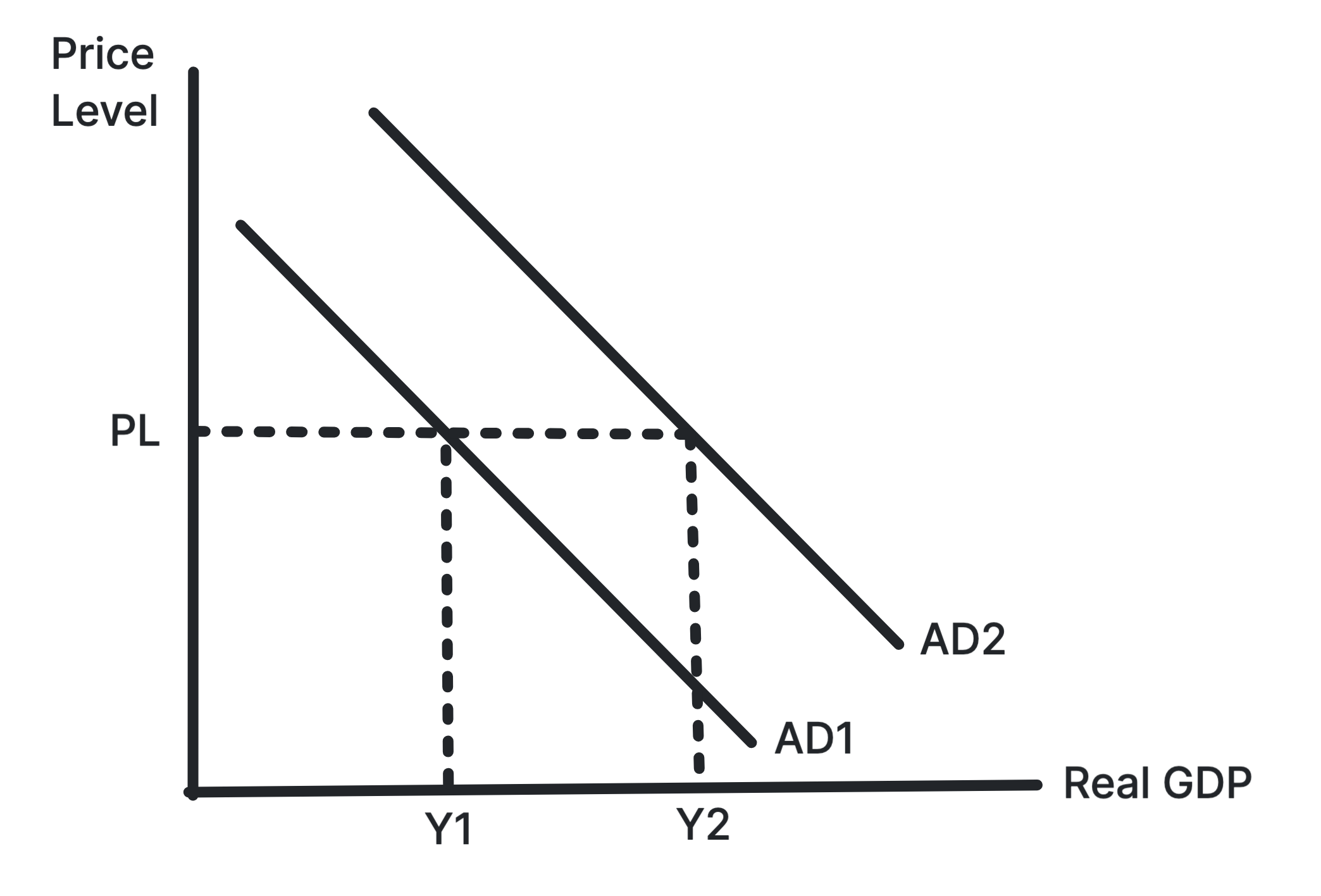
Changes in Aggregate Demand

Aggregate demand (AD): the total spending on an economy's goods and services at a given price level over a period of time: \[ AD = C + I + G + (X - M) \]

C is consumer spending, the largest part by far. I is investment by firms in capital such as machinery and buildings. G is government spending on goods and services, and X - M is exports minus imports.

A change in the price level moves the economy along the AD curve. Anything that changes C, I, G or X - M at every price level shifts the whole curve. AD shifts right when:

• Interest rates fall: borrowing is cheaper and saving pays less, so households spend more and firms invest more.
• Confidence rises: households expecting secure jobs spend more, and firms expecting strong sales invest.
• Fiscal policy loosens: the government spends more or cuts taxes, leaving households and firms more to spend.
• Exports rise: a weaker pound or faster growth abroad means more overseas buyers for UK goods.

Each one reversed shifts AD to the left.

Changes in Aggregate Supply

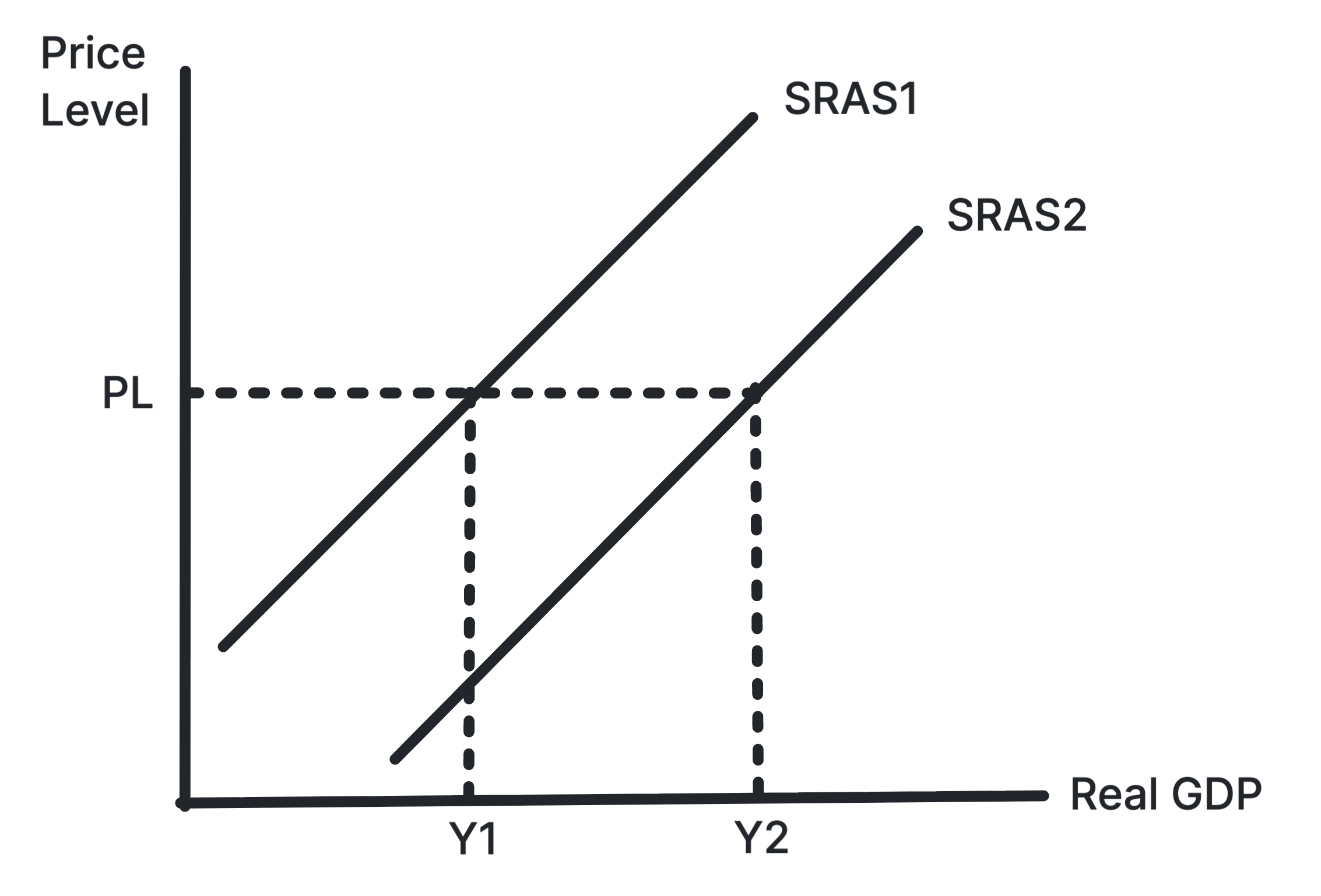
Short-run aggregate supply (SRAS): the total output firms in an economy plan to supply at each price level in the short run, when the prices of factors of production, such as wages, are fixed.

SRAS shifts when costs change across the economy. Lower wages, cheaper energy and raw materials, a stronger pound (cheaper imported inputs) or a cut in indirect taxes all shift SRAS right. A rise in any of them shifts it left: firms supply less at each price level.

Long-run aggregate supply (LRAS): the most an economy can produce when all its resources are fully and efficiently employed. It shows the economy's productive capacity.

LRAS shifts right when the economy gains more or better resources: more workers, better skills, more capital, new technology. This is long-run economic growth, and it is what supply-side policies aim for (unit 4.4.3).

Full Capacity Output

Full capacity output: the level of real GDP at which all of the economy's resources are in use, so output cannot rise any further in the short run.

Economists draw LRAS in two ways. In the classical view it is vertical at full capacity: the economy always returns there, so in the long run a change in AD moves only the price level. In the Keynesian view, shown in Figure 3, the economy can stay below full capacity for a long time.

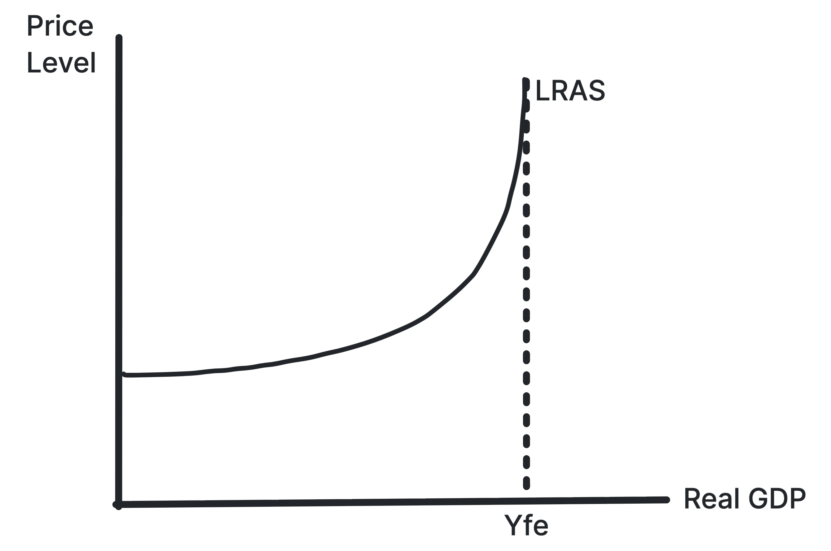
• The flat section: many workers and machines are idle, so firms can produce more without paying more for them. Output rises with no rise in prices.
• The rising section: spare capacity is running out, so firms bid for scarce workers and materials. Output still rises, but costs and prices rise too.
• The vertical section: the economy is at full capacity (Yfe). More spending only raises prices.

Effects on Inflation and Unemployment

Where the economy starts on the LRAS curve decides what a shift does to prices and jobs.

• AD rises with spare capacity: more spending → firms bring idle workers and machines back into use → output rises with little change in prices → unemployment falls and inflation barely moves.
• AD rises near full capacity: more spending → firms compete for scarce staff and materials → wages and costs rise → prices rise with little extra output. This is demand-pull inflation.
• AD falls: households and firms spend less → firms cut output → they need fewer workers → unemployment rises and inflation falls.
• SRAS shifts left: energy or wage costs rise → firms raise prices and cut output → cost-push inflation and higher unemployment at the same time, as when energy prices jumped in 2022.
• LRAS shifts right: productive capacity grows → output can rise without pushing up costs → growth with lower inflation, and more jobs if AD grows to match.

The effect depends on:

• Spare capacity: the same rise in AD cuts unemployment in a recession but mainly causes inflation in a boom.
• The size of the shift: a small change in spending can grow through the multiplier, below.
• Time: firms take time to hire, invest or raise prices, and in the classical view the economy returns to full capacity, so a rise in AD only lifts output for a while.

The Multiplier Effect

Multiplier effect: the process by which an initial change in spending leads to a larger final change in real GDP.

Spending by one person is income for another. If the government spends £1 billion on a new hospital, the builders spend part of what they earn in local shops, whose staff spend part of theirs. Each round is smaller, because some income leaks out as saving, tax or spending on imports.

The marginal propensity to consume (MPC) is the share of each extra pound spent on UK goods and services. The marginal propensity to withdraw (MPW) is the share that leaks out: the marginal propensities to save (MPS), pay tax (MPT) and import (MPM) added together. MPC + MPW = 1.

\[ \text{Multiplier} = \frac{1}{1 - \text{MPC}} = \frac{1}{\text{MPW}} \]

If households save 10p, pay 20p in tax and spend 10p on imports out of each extra pound, MPW is 0.4 and the multiplier is 1 ÷ 0.4 = 2.5. A £2 billion rise in government spending then raises real GDP by £5 billion.

The multiplier works in reverse too. A fall in spending, such as a factory closure, cuts other people's incomes and spending round after round. The multiplier is larger when:

• Leakages are small: low tax rates, little saving and few imports leave more of each pound to be spent again.
• There is spare capacity: firms can meet the extra demand with more output. Near full capacity much of it goes into higher prices.
• Confidence is high: people who feel secure spend extra income; worried households save it.

What the Model Shows About the Economy

The AD/AS model puts the main objectives on one diagram: real GDP shows growth, the price level shows inflation, and the gap between output and full capacity shows unemployment. That makes it useful in three ways:

• Finding the cause: inflation with rising output points to strong demand; inflation with falling output points to a supply shock.
• Choosing a policy: weak demand calls for demand-side policies (unit 4.4.2); low capacity calls for supply-side policies.
• Showing trade-offs: pushing AD up near full capacity buys a little growth at the cost of higher inflation.

It has limits. Classical and Keynesian economists disagree about the shape of LRAS, so the same policy can look effective on one diagram and useless on the other. The model shows the direction of a change, not its size or timing, and no one knows exactly where full capacity is.