Price Elasticity of Supply
Definition and Calculation
Price Elasticity of Supply (PES): Measures the responsiveness of quantity supplied to a change in the good's own price. It helps us understand how easily, quickly or cheaply producers can increase output when the price rises.
Formula:
Interpreting PES Values
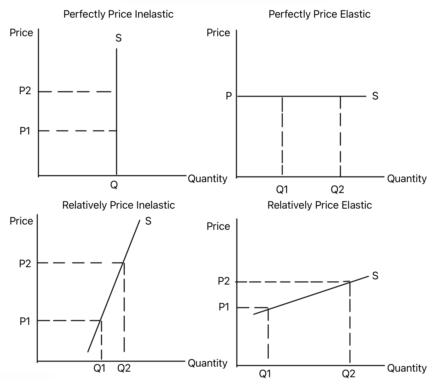
| PES Value | Classification | Description & Example |
|---|---|---|
| PES = 0 | Perfectly inelastic supply | Quantity supplied cannot change (e.g., fixed number of theatre seats on a given night). The supply curve is vertical. |
| 0 < PES < 1 | Relatively inelastic supply | The percentage change in quantity supplied is less than the percentage change in price (e.g., agricultural products, goods with complex production). |
| PES = ∞ | Perfectly elastic supply | The quantity supplied will fall to zero with any change in the price, but supply is unlimited at a specific price. |
| PES > 1 | Relatively elastic supply | The percentage change in quantity supplied is greater than the percentage change in price (e.g., manufactured goods like t-shirts). |
Worked Example: Why PES Depends on Time
A clothing manufacturer currently makes 4,000 t-shirts a month. The market price rises from £8 to £10, an increase of 25%. How much more it can supply depends on how long it has to respond:
| Time period | Output | % change in Qs | PES |
|---|---|---|---|
| Short run (existing factory) | 4,000 → 4,400 | \( \frac{400}{4{,}000} \times 100 = 10\% \) | \( \frac{10}{25} = 0.4 \) |
| Long run (extra machines and staff) | 4,000 → 6,000 | \( \frac{2{,}000}{4{,}000} \times 100 = 50\% \) | \( \frac{50}{25} = 2.0 \) |
The price change is identical in both rows - only the time available to respond differs. In the short run PES is 0.4, so supply is relatively inelastic; in the long run it is 2.0, so supply is relatively elastic. This is why the same good can sit in two different rows of the table above depending on the period under discussion.
Key Determinants of PES
The main factor influencing PES is time. The ability to increase supply is heavily constrained in the short run but improves in the long run.
Other Determinants:
| Determinant | Impact on PES |
|---|---|
| Spare Production Capacity | If a firm has unused capacity, supply can be increased quickly (elastic). If at full capacity, supply is inelastic. |
| Ease of Storing Stocks/Inventories | If goods can be stored cheaply, firms can release stocks to respond to price increases (elastic). |
| Mobility of Factors of Production | If resources (labour, capital) can be easily switched between products, supply is more elastic. |
| Complexity of Production | Simple, quick-to-produce goods have more elastic supply. Goods requiring rare materials or lengthy processes are inelastic. |
| Marginal Cost of Production | If the marginal cost of producing additional units is low, supply is more elastic. If marginal cost is high, supply is more inelastic. |
| Availability of Raw Materials | If raw materials are readily available, supply is more elastic. If they are scarce or difficult to obtain, supply is more inelastic. |
Short-Run vs. Long-Run Supply
Short Run: A period where at least one factor of production is fixed (e.g., factory size, number of machines). Supply is typically more price inelastic in the short run as firms cannot instantly expand all inputs.
Long Run: A period where all factors of production are variable. Firms can build new factories, hire more workers, etc. Supply is therefore more price elastic in the long run.
Stuck on this topic? Work through it with an online A-Level Economics tutor in a free 15-minute intro call, or send an essay on it for A-Level Economics essay marking.