Aggregate Demand and Aggregate Supply Analysis
What Is Aggregate Demand?
Definition: Aggregate demand is the total demand for all goods and services in an economy at a given average price level and in a given time period.
Formula (Expenditure Approach):
\[ AD = C + I + G + (X - M) \]
C = Consumption: Spending by consumers/households on goods and services.
I = Investment: Spending by firms on capital goods e.g. machinery, equipment, and factories.
G = Government Spending: Spending on state-provided goods and services. This excludes transfer payments such as benefits.
(X - M) = Net Exports: Exports minus imports.
The Components of AD and Their Relative Importance
- Consumption (C): Around 60% of AD. This is the largest component and is influenced by factors such as consumer confidence, disposable income, and interest rates.
- Investment (I): Around 14% of AD. This is the most volatile component and is influenced by business confidence, interest rates, and expectations of future economic conditions.
- Government Spending (G): Around 25% of AD. This is determined by government fiscal policy and can be influenced by political priorities and the state of the economy (e.g., during a recession, government spending may increase to stimulate demand).
- Net Exports (X - M): Usually a small and often negative percentage, roughly 1% or less. This is influenced by exchange rates, income levels in trading partner countries, and trade policies.
Implications: Because consumption is the largest component of AD, changes in consumer confidence, disposable income, and interest rates can have a more significant impact on aggregate demand than changes in investment or net exports.
The Aggregate Demand Curve
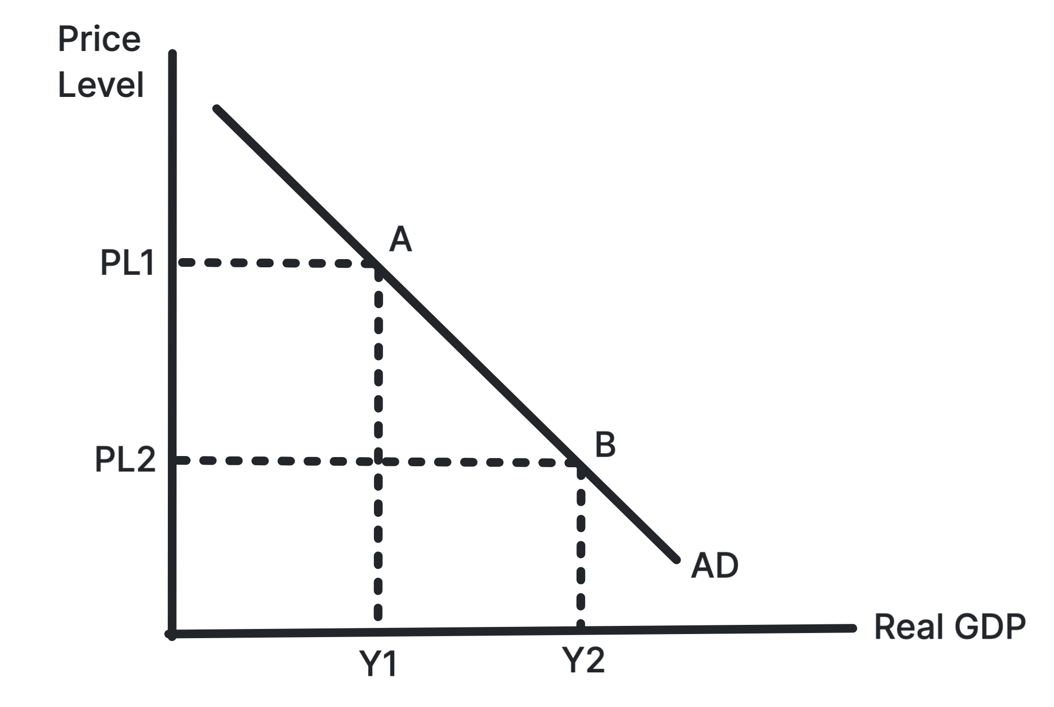
Why the AD Curve Slopes Downward
- Wealth Effect: As the price level falls, the real value of money increases, making consumers feel wealthier and more likely to spend, increasing consumption (C).
- Interest Rate Effect: A lower price level reduces the demand for money, leading to lower interest rates, which encourages borrowing and investment (I) and increases consumption (C).
- International Trade Effect: A lower domestic price level makes exports cheaper and imports more expensive, increasing net exports (X - M).
Movements vs. Shifts of the AD Curve
A Movement Along the AD Curve
- Cause: A change in the average price level, assuming other factors stay constant.
- This shows how the quantity of real GDP demanded changes with the price level.
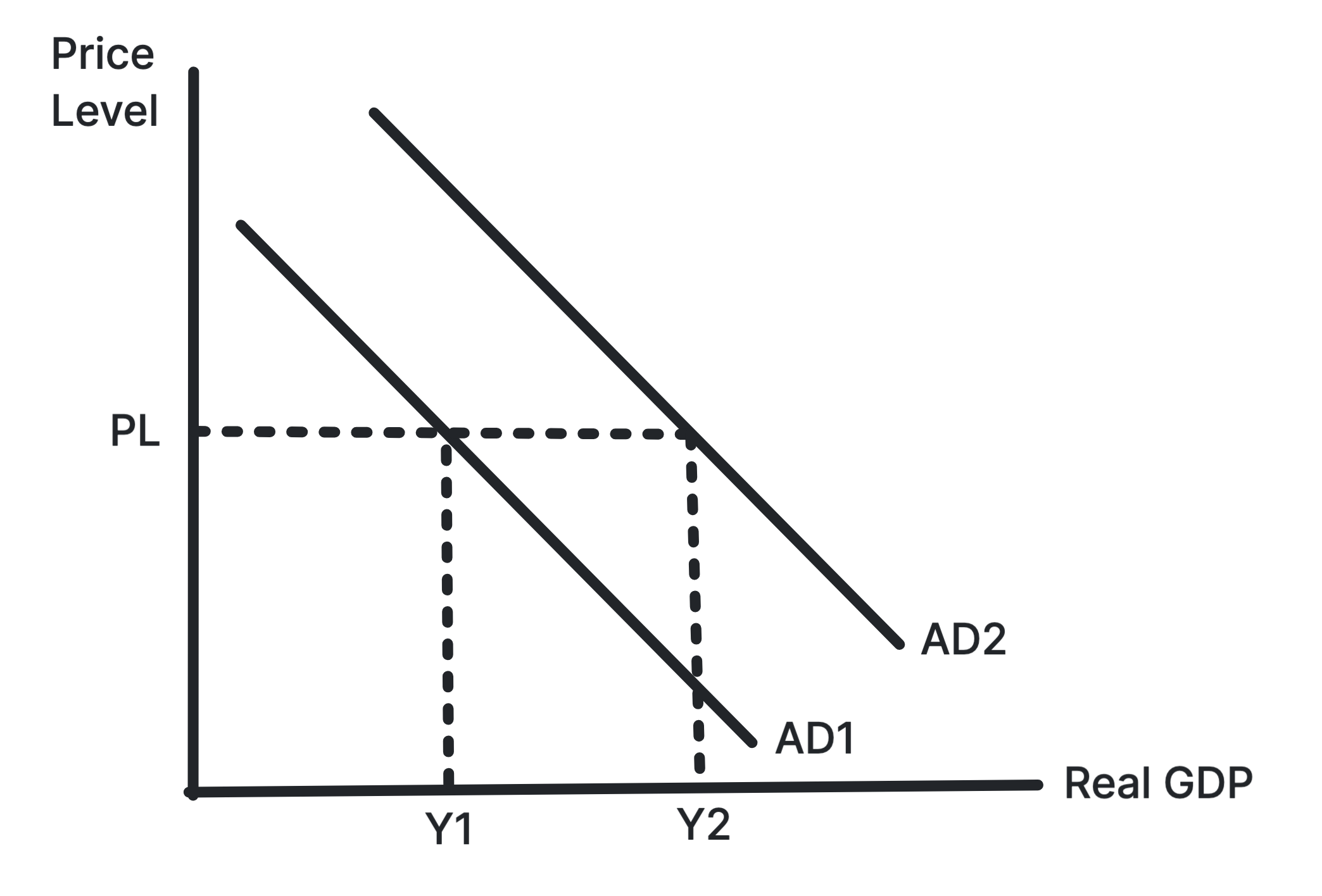
A Shift of the Entire AD Curve
- Cause: A change in any determinant of AD other than the price level, meaning a change in C, I, G, or X - M.
- This changes total planned expenditure at every given price level.
Determinants of AD
| Component | Affected by |
|---|---|
| Consumption (C) |
|
| Investment (I) |
|
| Government Spending (G) |
|
| Net Exports (X - M) |
|
The SRAS Curve
Definition: Short-run aggregate supply is the total planned output of goods and services in an economy at a given price level, assuming that at least one factor of production, such as capital or technology, is fixed.
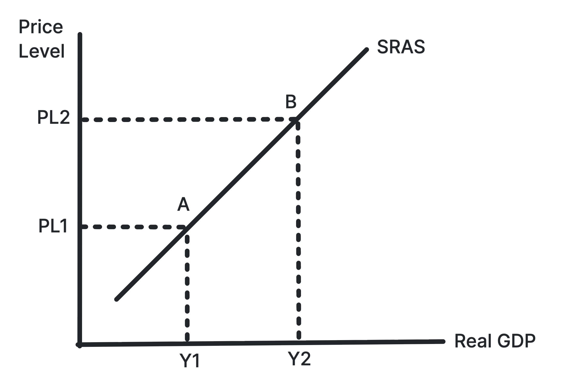
The SRAS curve is upward sloping because, in the short run, higher output leads to higher unit costs, such as overtime wages. Firms therefore need a higher price to make additional production worthwhile.
Movements vs. Shifts of the SRAS Curve
A Movement Along the SRAS Curve
- Cause: A change in the average price level, holding other things constant.
- This shows firms changing their level of output in response to a change in price level.
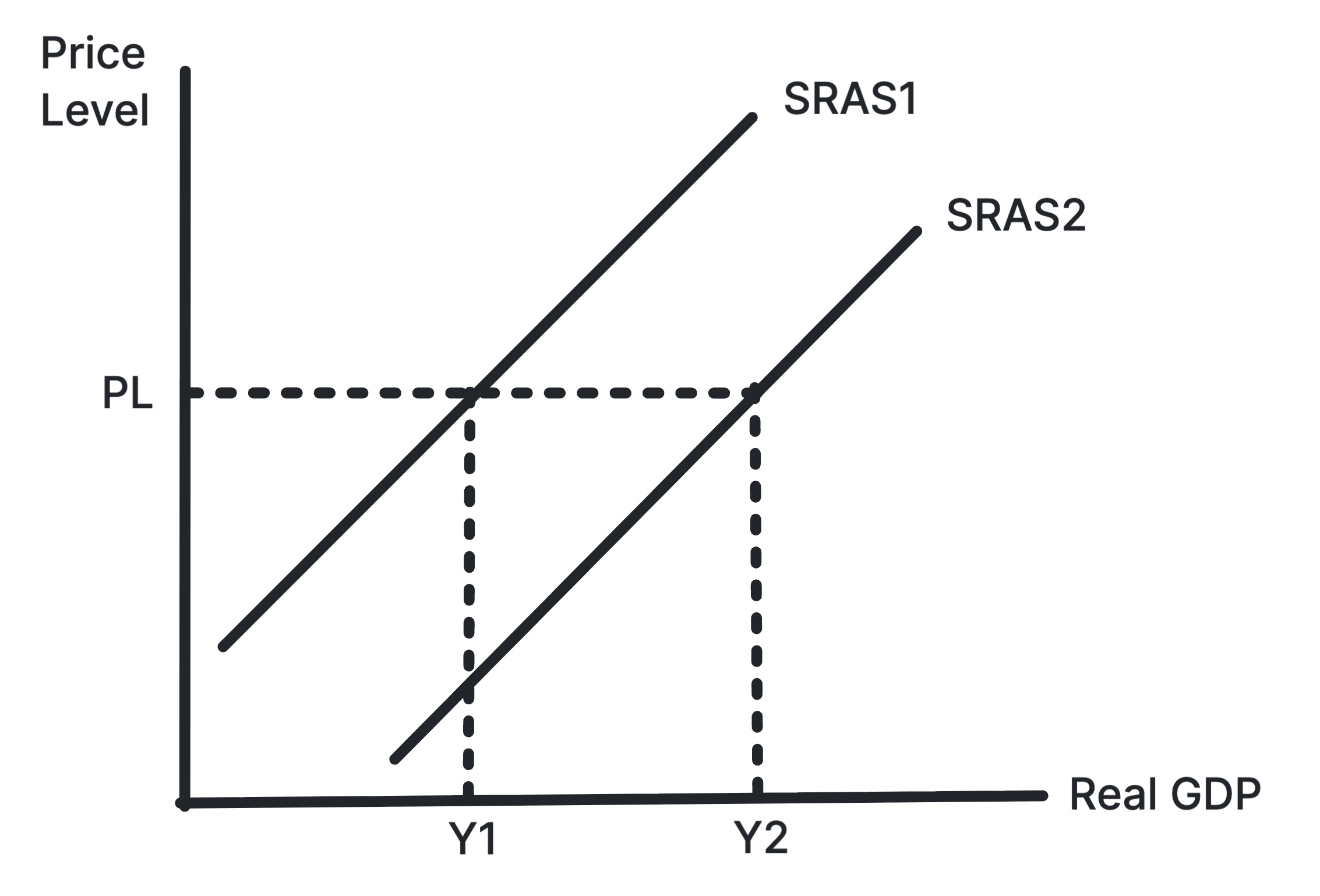
A Shift of the Entire SRAS Curve
- Cause: A change in any condition of SRAS, meaning a change in production costs for firms across the economy.
- This changes the level of output firms are willing to supply at every given price level.
Key Factors Influencing SRAS
| Factor | Impact on SRAS |
|---|---|
| Cost of Raw Materials or Energy | A fall in the cost of raw materials or energy reduces production costs, shifting SRAS to the right. A rise in costs shifts SRAS to the left. |
| Labour Costs | A fall in labour costs reduces production costs, shifting SRAS to the right. A rise in labour costs shifts SRAS to the left. |
| Exchange Rates | A depreciation of the domestic currency makes imported raw materials more expensive, raising production costs and shifting SRAS to the left. An appreciation has the opposite effect. |
| Indirect Taxes | An increase in indirect taxes raises production costs, shifting SRAS to the left. A decrease in indirect taxes lowers production costs, shifting SRAS to the right. |
| Subsidies | Government subsidies can lower production costs, shifting SRAS to the right. The removal of subsidies can raise costs, shifting SRAS to the left. |
| Supply Shocks | Unexpected events, such as natural disasters or sudden changes in oil prices, can affect production costs and shift SRAS. A negative supply shock shifts SRAS to the left, while a positive supply shock shifts it to the right. |
Long-Run Aggregate Supply (LRAS)
Definition: Long-run aggregate supply is the total potential output of an economy when all factors of production are fully and efficiently employed.
It represents the economy's productive capacity.
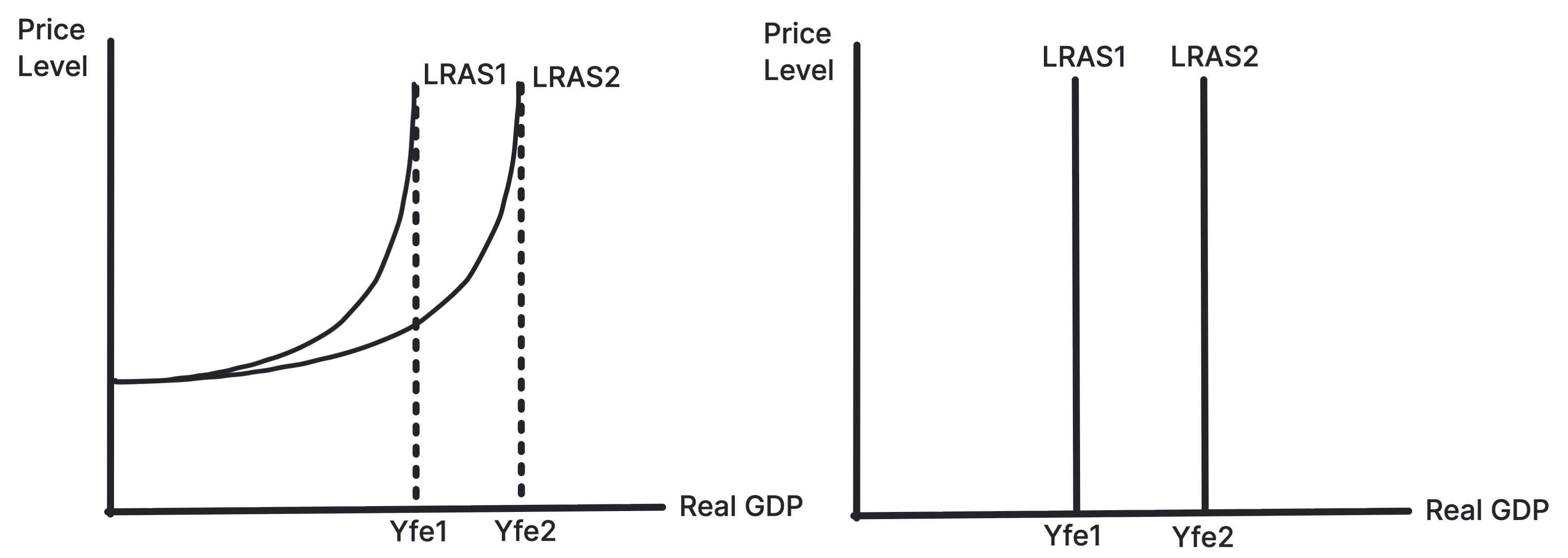
Key Idea: Shifts in LRAS represent long-run economic growth or decline, which is equivalent to an outward or inward shift of the production possibility frontier.
Two Views of the LRAS Curve
Economists disagree about the shape of the LRAS curve, leading to two main models.
The Classical View
Belief: In the long run, the economy will always adjust to full employment, so the level of output is determined by the quantity and quality of the factors of production, not by the price level.
The Curve: LRAS is perfectly inelastic, so it is vertical at the level of output corresponding to full employment, Yfe.
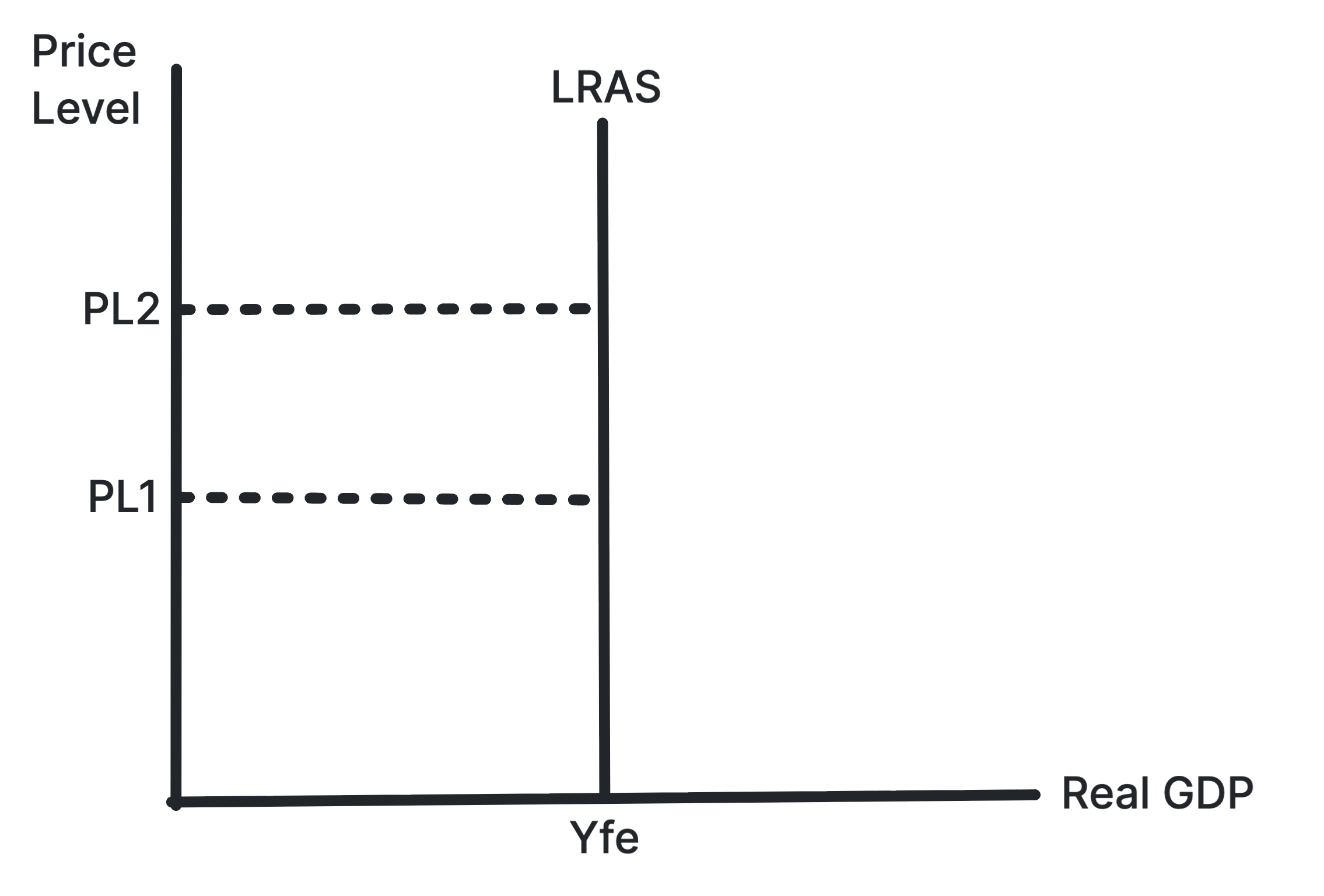
Analysis: In this view, any change in aggregate demand changes only the price level in the long run, not the level of real output.
The Keynesian View
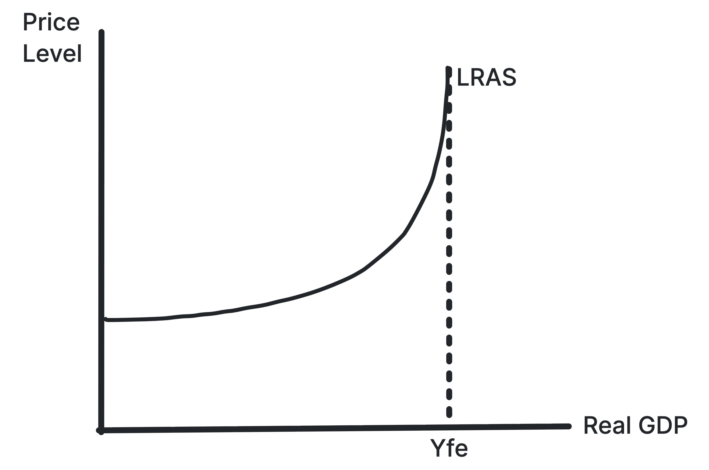
Belief: The economy can be below full employment for a long time, so the level of output can be influenced by aggregate demand in the long run, especially when there is spare capacity.
The Curve: LRAS is non-linear and often shown as L-shaped.
- It is perfectly elastic at low output where there is large spare capacity. This is because firms can increase output without increasing costs or prices due to the availability of unemployed resources.
- It becomes upward sloping as the economy approaches capacity and inflationary pressures build. This is because resources have become scarcer, so firms face rising costs to employ the remaining resources and pass these on to consumers in the form of higher prices.
- It becomes vertical at full capacity output, Yfe. This is because all resources are fully employed, so any further increase in aggregate demand will only lead to higher prices, not higher output.
Factors Influencing LRAS
Any change in the quantity or quality of the factors of production, including land, labour, capital, and enterprise, will shift LRAS and change the economy's productive potential.
| Factor | Effect on LRAS | Example |
|---|---|---|
| Technological Advances | Improve the quality of capital and make production more efficient. | AI, automation, and new manufacturing techniques. |
| Changes in Education and Skills | Improve the quality of labour and create a more productive workforce. | Greater spending on training and higher education. |
| Changes in Productivity | Increase output per worker or per hour, allowing more to be produced from the same inputs. | Better management and improved production processes. |
| Demographic Changes and Migration | Increase the quantity of labour and expand the working-age population. | Positive net migration or a rising birth rate. |
| Increase in Capital Stock | Increase the quantity of capital, such as machinery and infrastructure. | High levels of investment by firms and government. |
| Competition Policy and Deregulation | Improve efficiency and encourage enterprise and innovation. | Breaking up monopolies and reducing barriers to entry. |
| Institutional Improvements | Improve the quality of institutions and encourage investment. | Stronger property rights and lower corruption. |
Stuck on this topic? Work through it with an online A-Level Economics tutor in a free 15-minute intro call, or send an essay on it for A-Level Economics essay marking.