Perfect Competition
These Edexcel A-Level Economics revision notes cover unit 3.4.2, setting out the assumptions of perfect competition, the short-run and long-run equilibrium positions of competitive firms, and the efficiency properties that make perfect competition a benchmark for market analysis.
Key Characteristics
- There are many buyers and sellers.
- Products are homogeneous or identical.
- There is perfect information.
- There are no barriers to entry or exit.
- Firms are price takers, so they accept the market price.
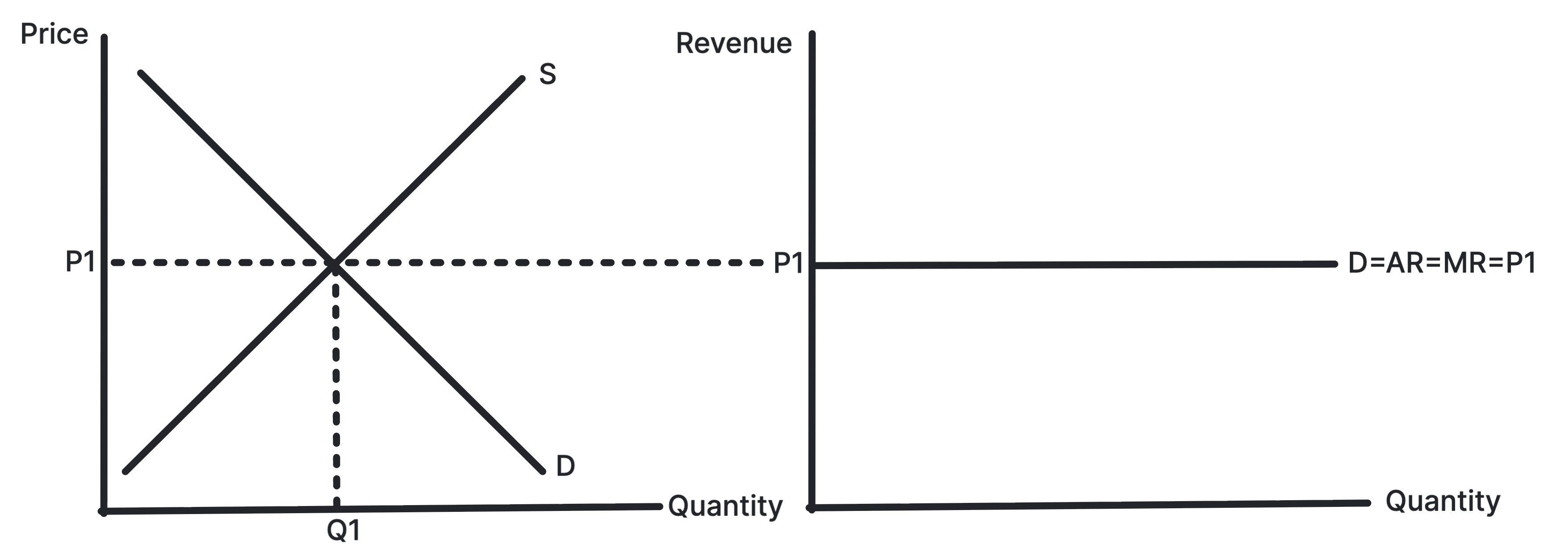
The Firm's Demand Curve
Because firms in perfect competition are price takers, the demand curve facing an individual firm is perfectly elastic, so it is horizontal.
This means \( P = MR = AR \).
The market price itself is determined by industry supply and demand.
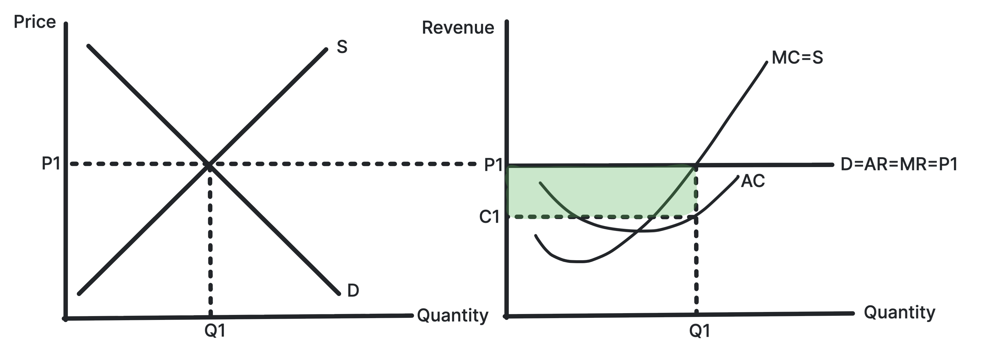
Short-Run Equilibrium: Profit and Loss
The firm maximises profit where \( MC = MR \).
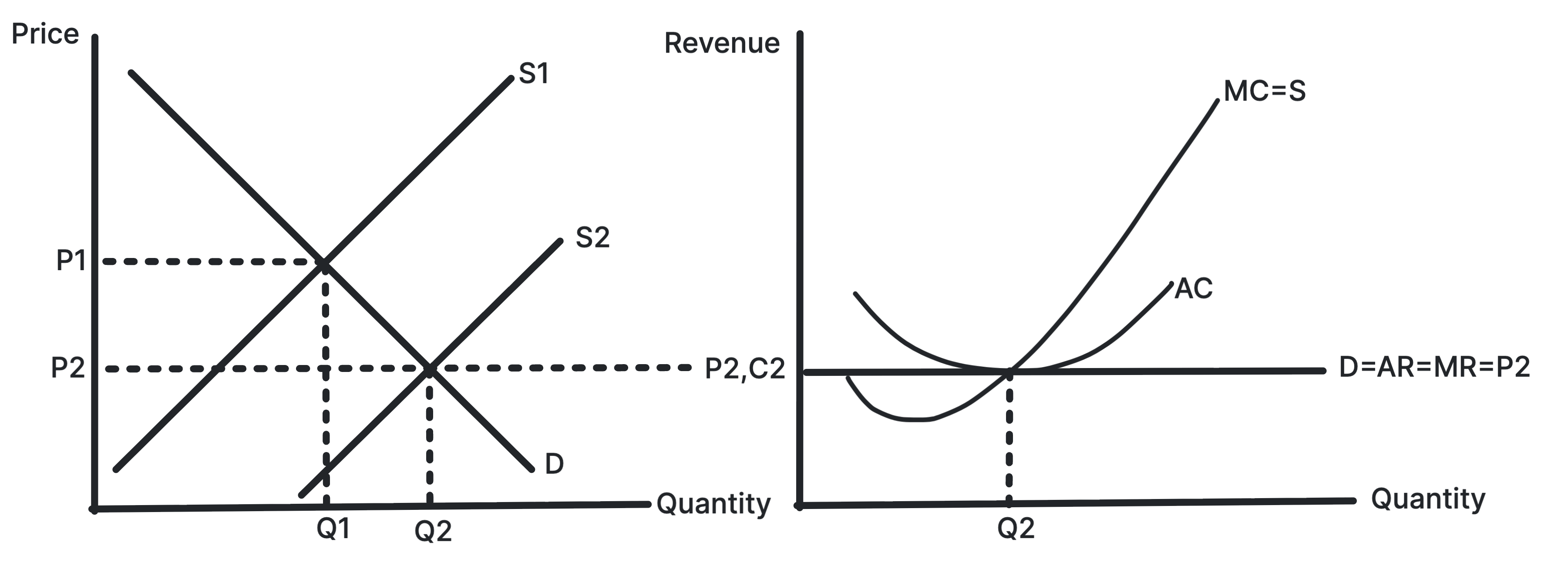
Long-Run Equilibrium: Normal Profit Only
Because there is freedom of entry and exit, perfect competition moves to a long-run equilibrium where firms earn only normal profit, so \( AR = AC \).
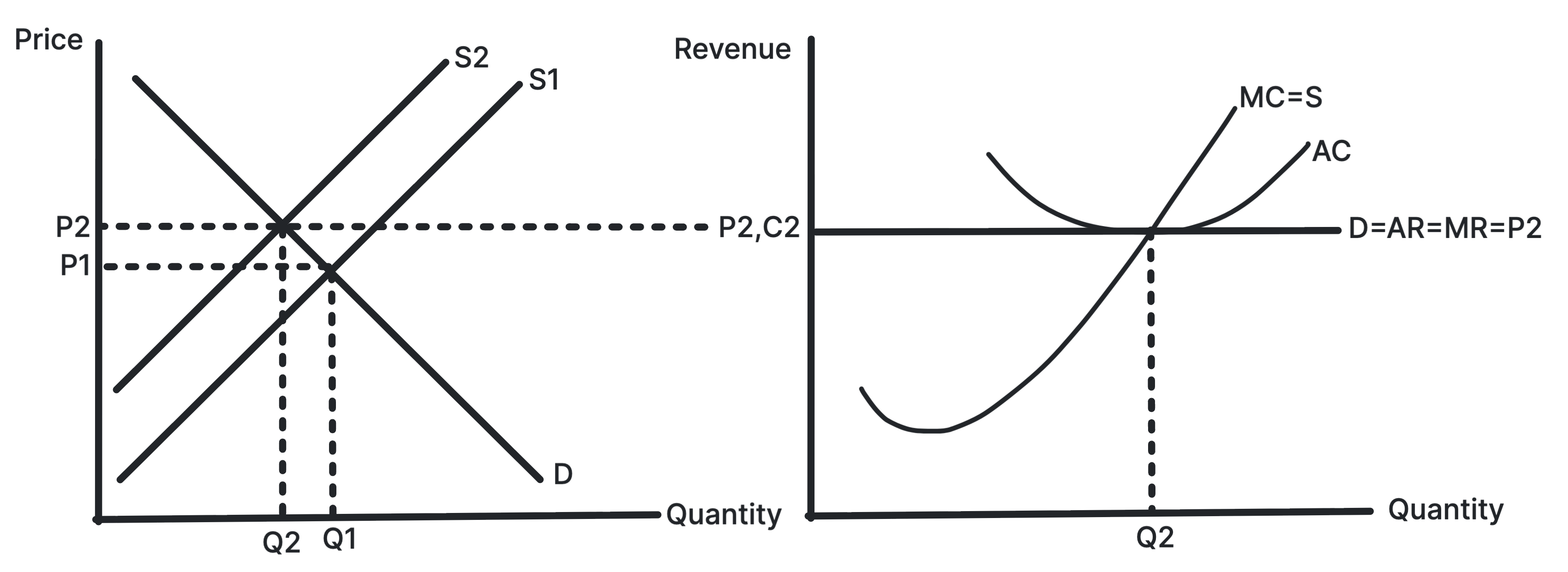
From Short-Run Supernormal Profit to Long-Run Equilibrium
- In the short run, firms may make supernormal profit.
- These profits attract new firms into the industry.
- Industry supply increases and shifts to the right.
- The market price falls.
- The firm's horizontal demand curve falls until it becomes tangent to the minimum point of the AC curve.
- At this point, \( P = AR = AC = MC \) and supernormal profit is eliminated.
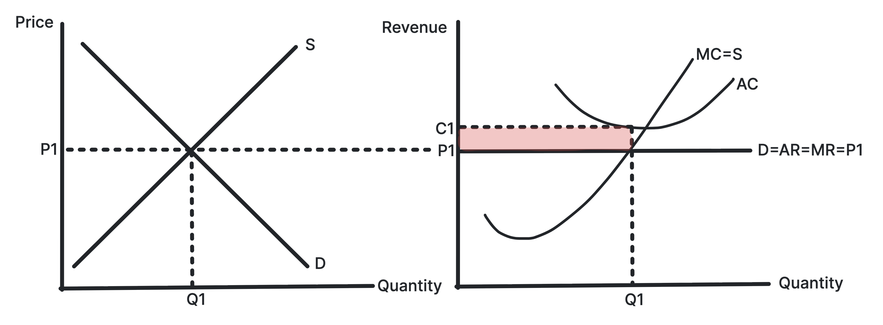
From Short-Run Loss to Long-Run Equilibrium
- In the short run, firms may make losses.
- Some firms leave the industry.
- Industry supply decreases and shifts to the left.
- The market price rises.
- Price rises until the firm's demand curve is tangent to the minimum point of AC and firms earn normal profit.
Efficiency in Long-Run Equilibrium
Productive efficiency: Yes, because the firm produces at minimum AC.
Allocative efficiency: Yes, because \( P = MC \).
Dynamic efficiency: Unlikely, because firms do not earn supernormal profit to fund research and development.
Exam Preparation
- List the characteristics of perfect competition.
- Draw the firm's horizontal demand curve and explain why it has that shape.
- Illustrate short-run supernormal profit and loss, and explain the adjustment process to long-run normal profit using industry supply shifts.
- Identify the long-run equilibrium point on the firm's diagram, where \( P = MC = \text{min AC} \).
- Analyse the efficiency of perfect competition in the long run.