Costs
Key Definitions
Fixed Costs (FC): Costs that do not vary with output, such as rent and salaries.
Variable Costs (VC): Costs that vary directly with output, such as raw materials and hourly wages.
Total Cost (TC): \( TC = TFC + TVC \)
Average Cost (AC): \( AC = \frac{TC}{Q} \)
Average Fixed Cost (AFC): \( AFC = \frac{TFC}{Q} \)
Average Variable Cost (AVC): \( AVC = \frac{TVC}{Q} \)
Marginal Cost (MC): \( \frac{\Delta TC}{\Delta Q} \), which is the additional cost incurred when producing one more unit.
Worked Example: Building a Cost Schedule
A bakery has fixed costs of £100 a day for rent and insurance. Its variable costs rise with output:
| Output | TFC | TVC | TC | AC | MC |
|---|---|---|---|---|---|
| 10 | £100 | £60 | £160 | £16.00 | — |
| 20 | £100 | £100 | £200 | £10.00 | £4.00 |
| 30 | £100 | £160 | £260 | £8.67 | £6.00 |
| 40 | £100 | £260 | £360 | £9.00 | £10.00 |
TC is TFC plus TVC, AC is TC divided by output, and MC is the change in TC divided by the change in output - so between 30 and 40 units MC is \( \frac{360 - 260}{40 - 30} = £10 \). Notice that AC bottoms out at £8.67 and then rises: AC turns upward exactly where MC rises above it.
Short-Run Cost Curves and Diminishing Returns
In the short run, at least one factor of production is fixed. For example, a firm may have a fixed amount of capital (machinery) but can vary the amount of labour it employs.
Adding more variable factors, such as labour, will initially increase productivity, but eventually diminishing marginal returns set in.
Diminishing Marginal Returns: The phenomenon where adding more of a variable input (like labour) to a fixed input (like machinery) results in smaller increases in output after each input is added. This is because the fixed input becomes a constraint, leading to inefficiencies.
For example, if a pub has a fixed number of bar counters, adding more bartenders will eventually lead to overcrowding and reduced efficiency, as they get in each other's way.
This concept is responsible for the shape of the Marginal Cost curve. Initially, as more labour is added, productivity increases, causing MC to fall. However, eventually diminishing marginal returns set in, and adding more units of labour leads to higher costs of increasing output.
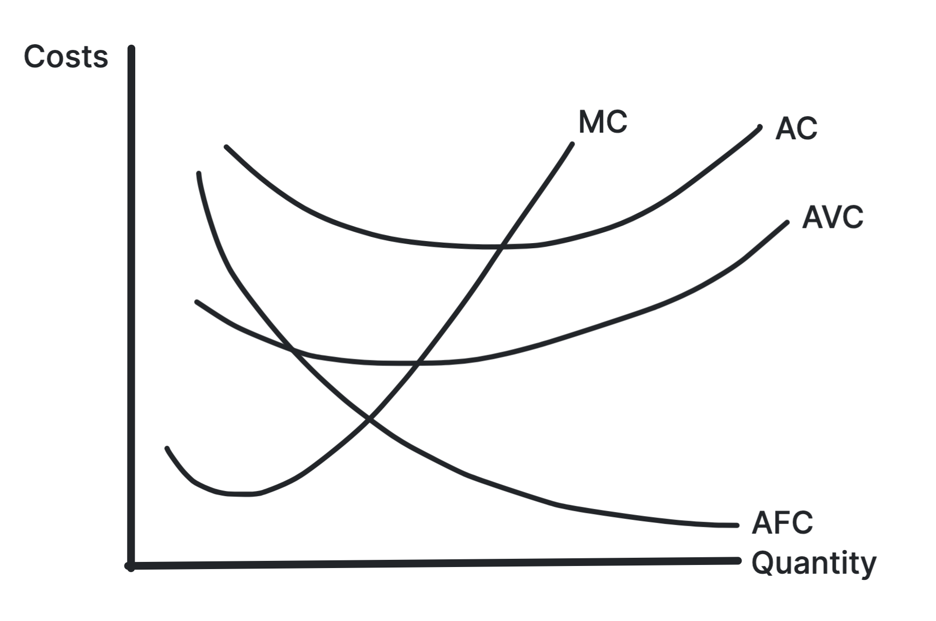
Why Are the Short-Run Curves U-Shaped?
- Initially: Increasing returns and specialisation pull MC, AVC, and AC down.
- Eventually: Diminishing returns cause MC to rise, which then pulls up AVC and AC.
The Relationship Between MC, AVC, and AC
When \( MC < AVC \), marginal cost pulls AVC down.
When \( MC > AVC \), marginal cost pulls AVC up.
This is why the MC curve intersects AVC at its minimum point. The same logic applies to the AC curve. This is the point where the firm is maximising productive efficiency.
Long-Run Average Cost (LRAC)
In the long run, all factors are variable, so the firm can change its scale of production.
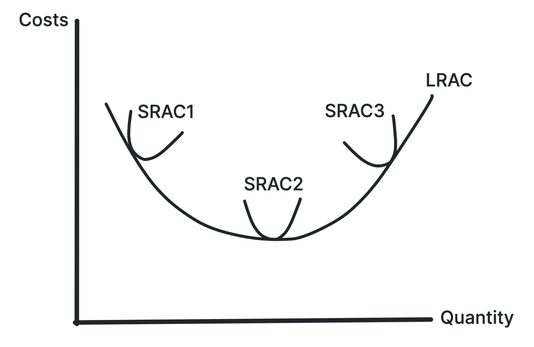
Why Is LRAC U-Shaped?
- Economies of scale (Increasing Returns to Scale): As output rises, LRAC falls due to factors such as, bulk buying, and spreading fixed costs over more units.
- Diseconomies of scale (Decreasing Returns to Scale): Beyond a certain output, LRAC rises because of managerial inefficiencies and coordination problems.
The Relationship Between SRAC and LRAC
- The LRAC curve is an envelope curve that touches each SRAC curve at the output where that scale is the cheapest available.
- Each SRAC curve represents a different scale of production, and the firm can move between them in the long run by adjusting all inputs.
- The LRAC curve is flatter than the SRAC curves because firms can adjust all inputs in the long run, allowing them to avoid the inefficiencies that cause the SRAC curves to rise.
Stuck on this topic? Work through it with an online A-Level Economics tutor in a free 15-minute intro call, or send an essay on it for A-Level Economics essay marking.