Written by
Eliot King— First-Class BSc (Hons) Economics, University of Bath · 6+ years teaching A-Level Economics · Edexcel A, Edexcel B, AQA and OCR
Specification Coverage: Edexcel unit 2.4.3 -
Equilibrium Levels of Real National Output. Students should be
able to understand and explain short-run and long-run
macroeconomic equilibrium, compare the Classical and Keynesian
views of equilibrium, analyse changes in AD and LRAS, identify
output gaps, and evaluate the policy implications of different
macroeconomic models.
Macroeconomic Equilibrium
Short-run equilibrium: This occurs where
aggregate demand equals
short-run aggregate supply. It determines the actual price level and
real national output.
Long-run equilibrium (Classical view): This
occurs where AD = SRAS = LRAS at the
full employment level of output,
Yfe.
The Two Views of Long-Run Equilibrium
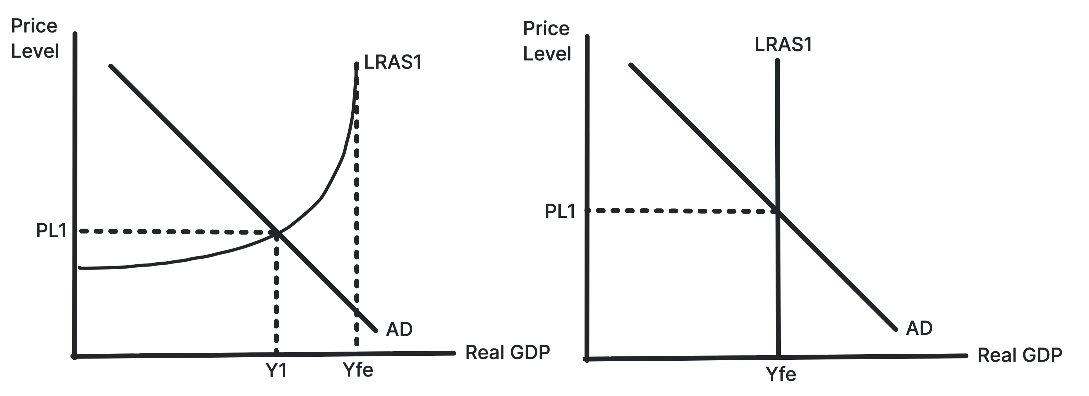
Figure 1: The AD-LRAS model illustrates the different views of
long-run equilibrium. The Classical model has a vertical LRAS,
while the Keynesian model has an L-shaped LRAS, allowing for
equilibrium at various output levels depending on AD.
Classical Equilibrium
In the Classical model, LRAS is vertical at
Yfe, and equilibrium can only occur at that
point. Any deviation from Yfe is temporary, as the economy will
self-correct through changes in wages and prices.
Keynesian Equilibrium
In the Keynesian model, LRAS is L-shaped,
allowing for equilibrium at various output levels below
Yfe. This means that the economy can be in
equilibrium with unemployment and unused capacity, and may not
self-correct without government intervention.
Aggregate Demand shifts: The Classical View
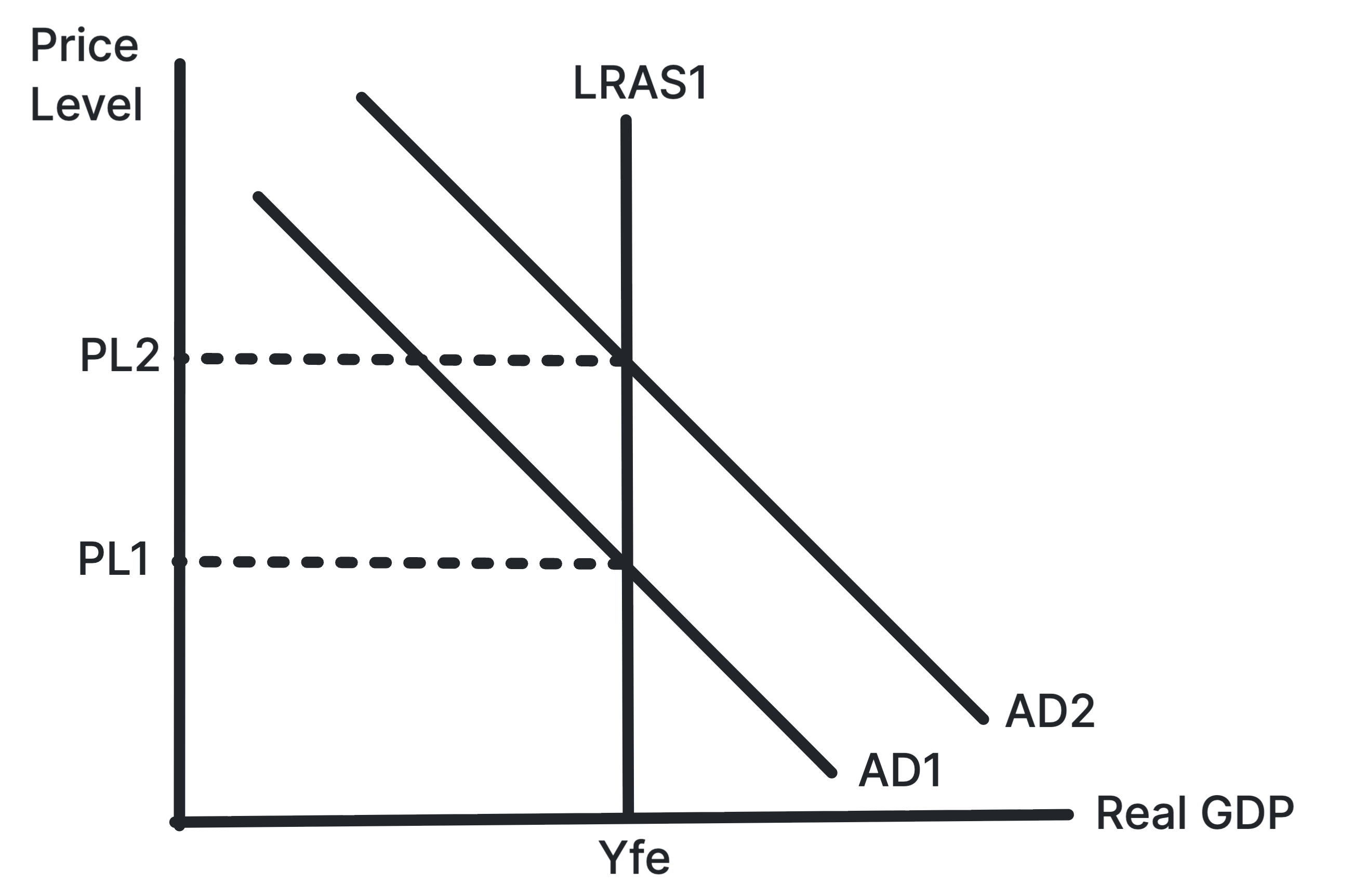
Figure 2: An increase in AD (AD1 to AD2) in the Classical
model leads to a higher price level (P1 to P2) but no change
in output (Yfe).
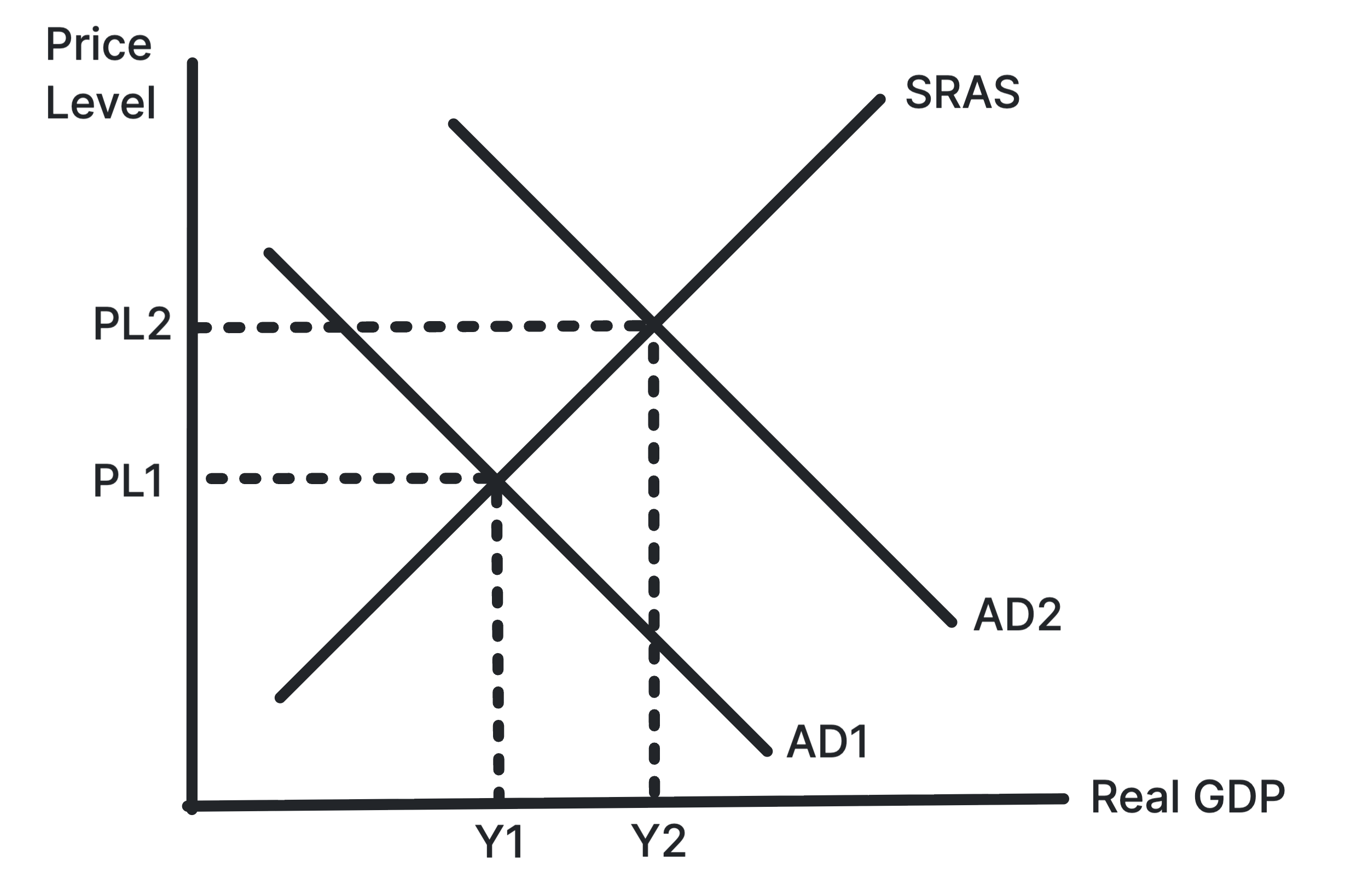
Figure 3: An increase in AD (AD1 to AD2) in the SRAS-AD model
leads to a higher price level (P1 to P2) and an increase in
output (Y1 to Y2) in the short run.
Aggregate Demand shifts: The Keynesian View
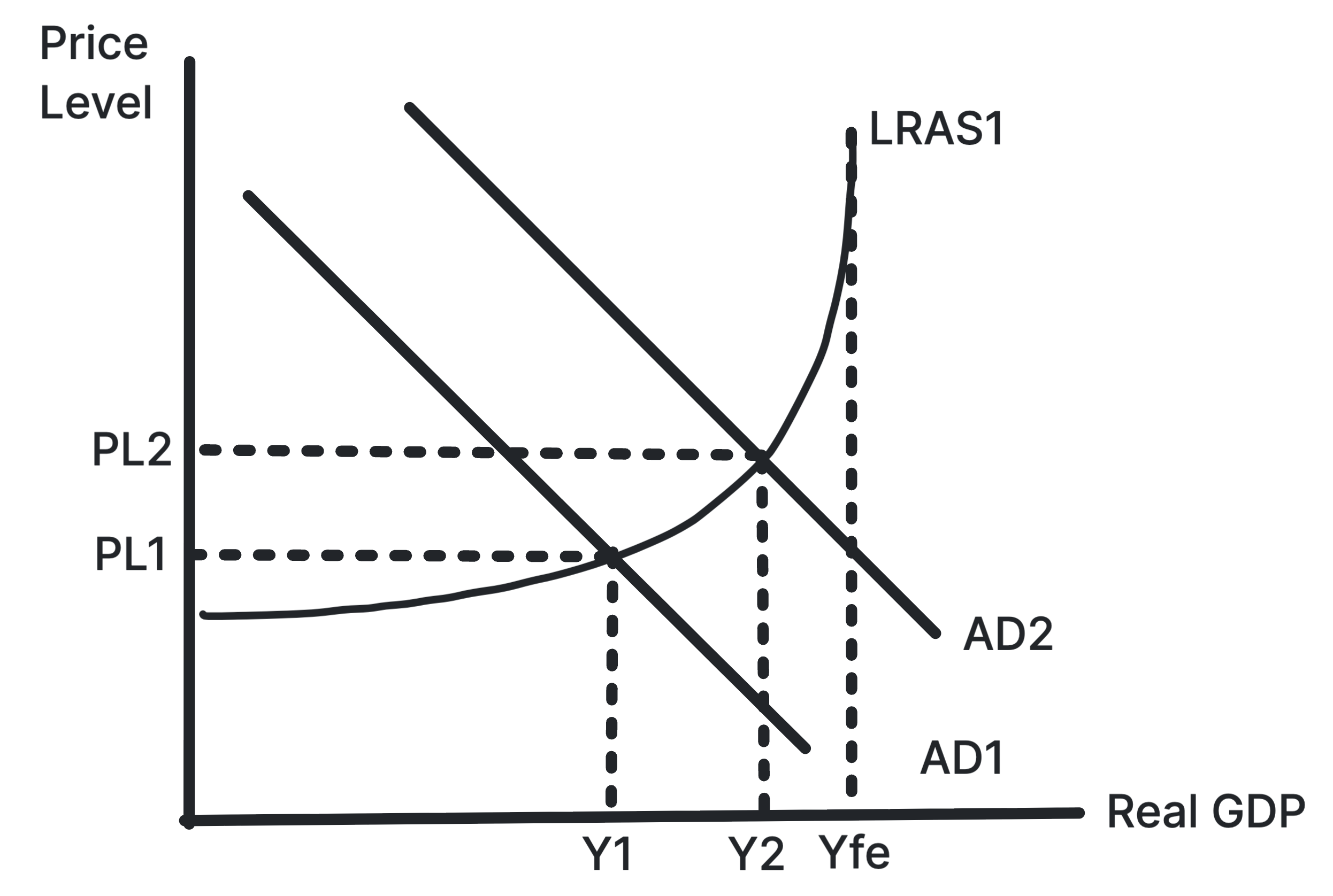
Figure 4: An increase in AD (AD1 to AD2) in the Keynesian
model can lead to a significant increase in output (Y1 to Y2)
without a rise in the price level when the economy is
operating in the horizontal section of the LRAS curve.
Key Insight: The effect of an AD shift depends
on where the economy is operating on the LRAS curve, especially
whether there is spare capacity or full capacity.
Shifts in Long-Run Aggregate Supply
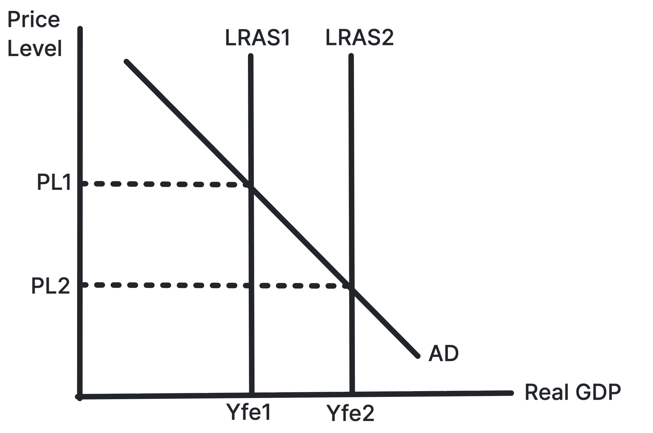
Figure 5: An increase in LRAS (LRAS1 to LRAS2) in the
Classical model leads to a higher potential output (Yfe1 to
Yfe2) and a lower price level (P1 to P2) in the long run.
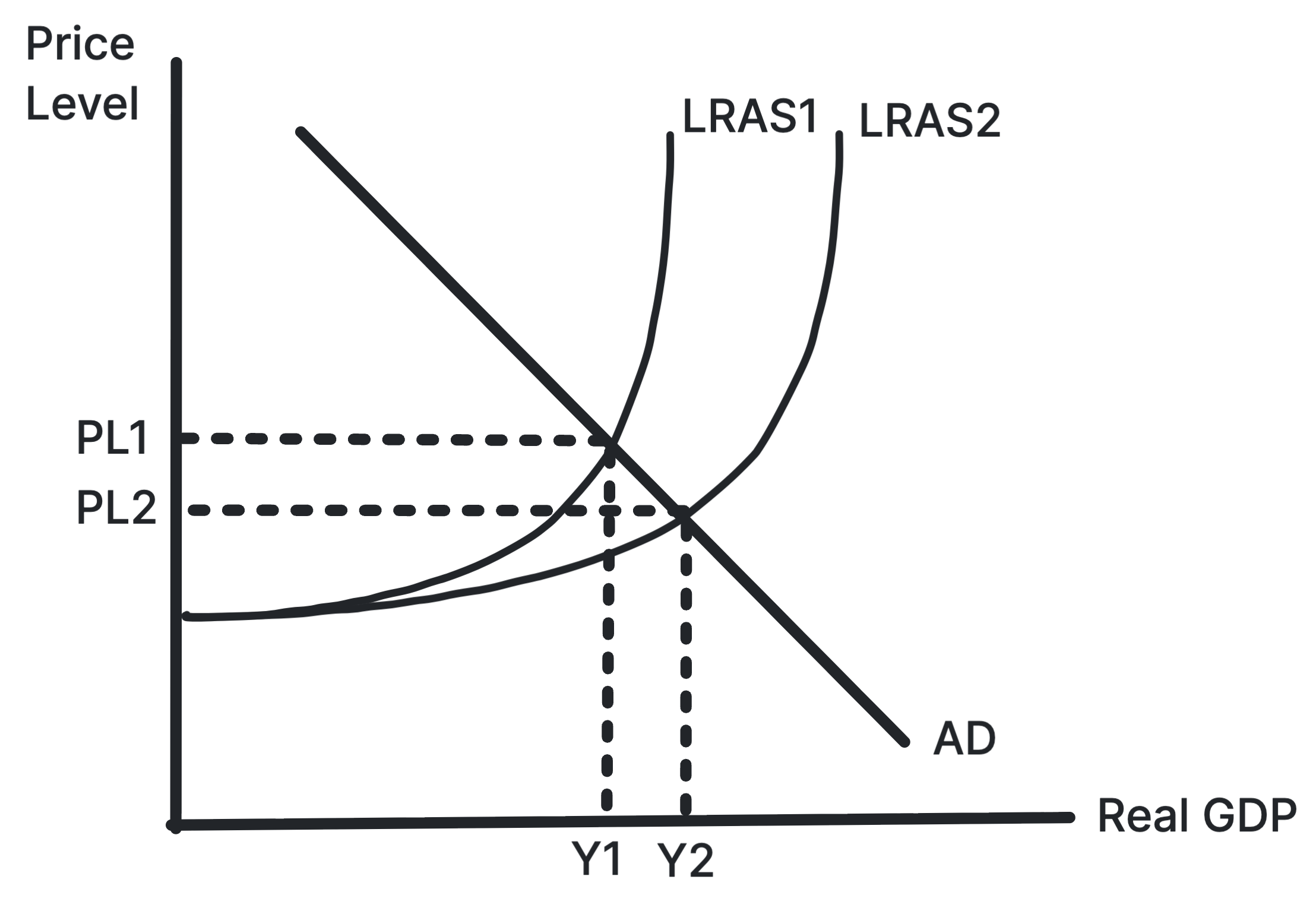
Figure 6: An increase in LRAS (LRAS1 to LRAS2) in the
Keynesian model can lead to a higher output (Y1 to Y2) and a
lower price level (P1 to P2) in the long run, especially if
the economy was previously operating in the vertical section
of the LRAS curve.