Price Determination
These Edexcel A-Level Economics revision notes cover unit 1.2.6, explaining how the interaction of demand and supply determines equilibrium price and quantity, how shocks create disequilibrium, and how markets adjust back to equilibrium.
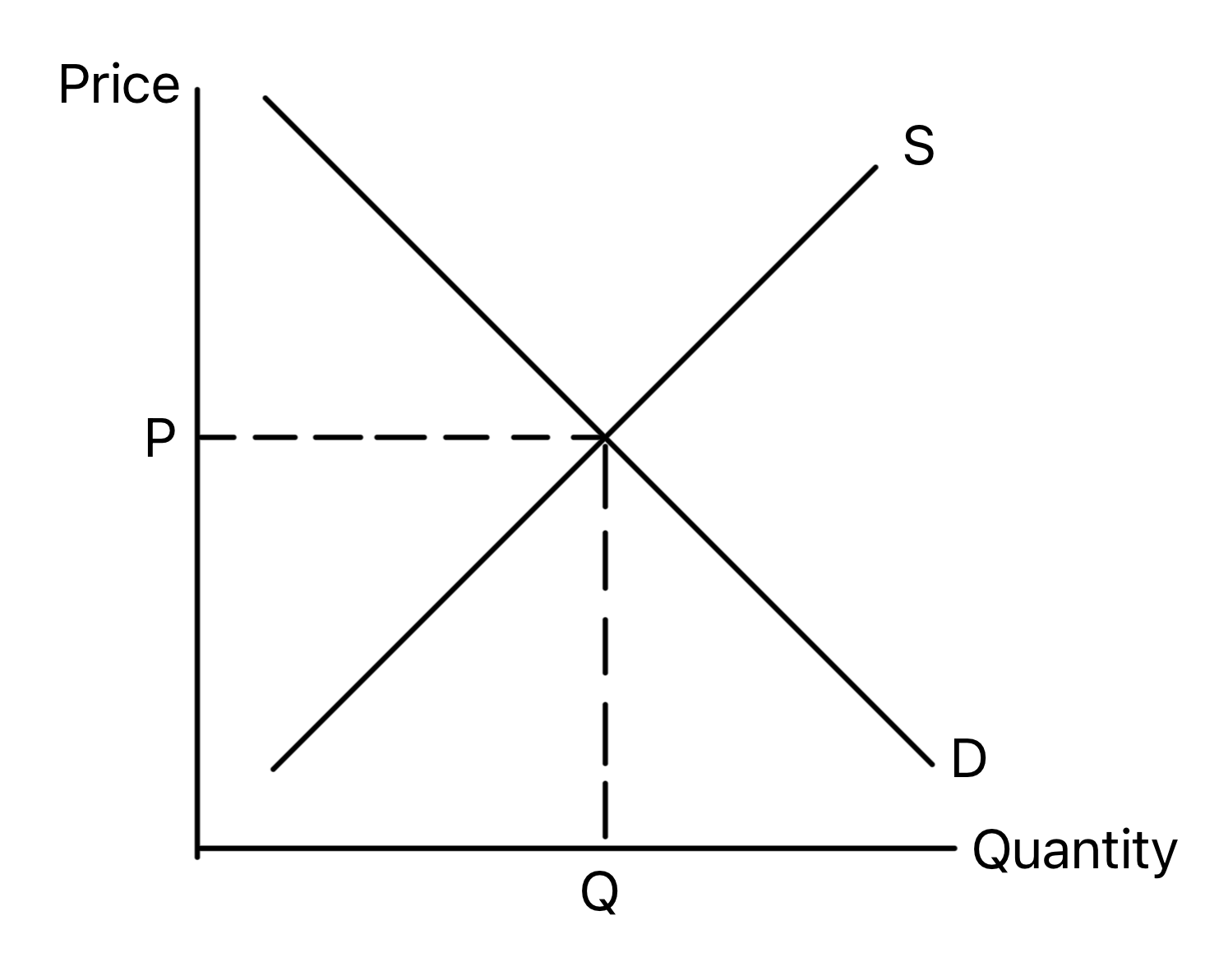
Market Equilibrium
Market Equilibrium: The point where market demand equals market supply.
Equilibrium Price (Market Clearing Price): The price where there is no excess demand or supply. The market 'clears'.
Equilibrium Quantity: The quantity bought and sold at the equilibrium price.
Disequilibrium
Markets are dynamic (constantly changing). Any change in conditions creates disequilibrium, but competitive market forces push the price back towards equilibrium.
a) Excess Demand (Shortage)
Occurs when: Price is below the equilibrium price (P1).
Result: Quantity Demanded (QD) > Quantity Supplied (QS).
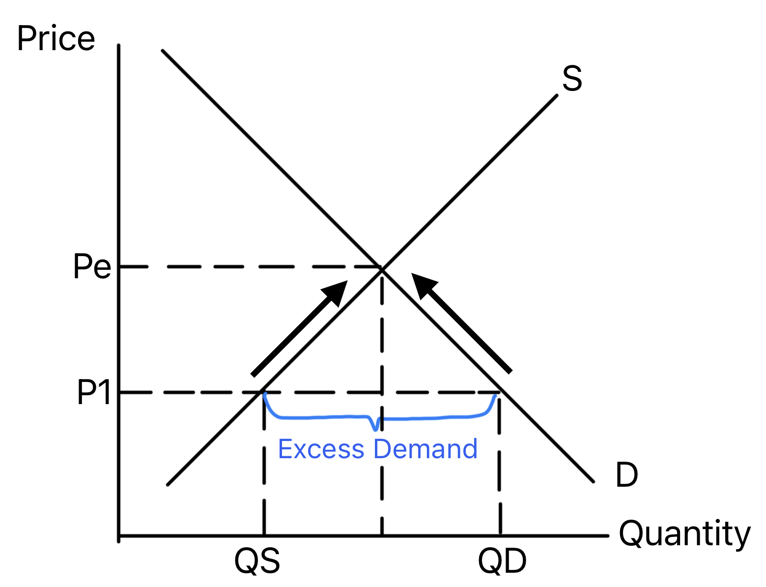
Market Correction: The shortage creates competition among buyers, giving sellers the power to raise prices. As price rises:
- Extension in QS (movement up supply curve).
- Contraction in QD (movement up demand curve).
This continues until a new equilibrium is reached.
b) Excess Supply (Surplus)
Occurs when: Price is above the equilibrium price (P1).
Result: Quantity Supplied (QS) > Quantity Demanded (QD).
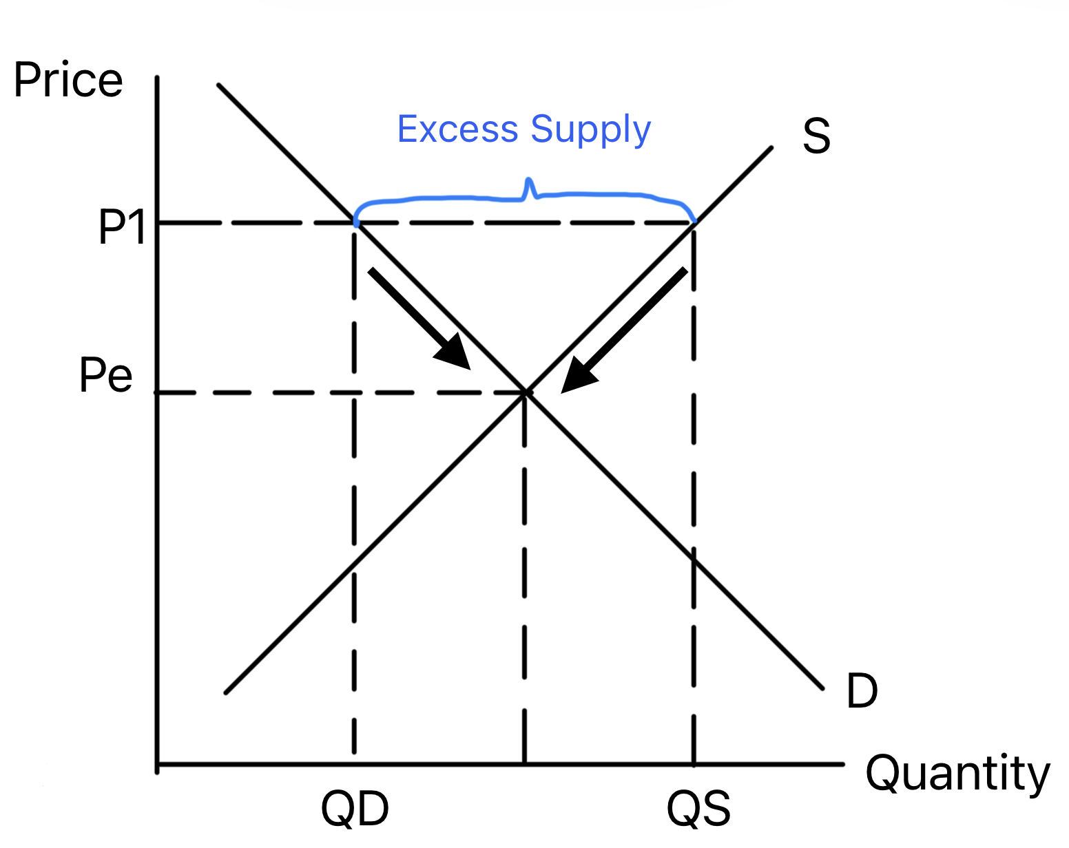
Market Correction: The surplus means sellers have unsold stock, leading them to lower prices to compete. As price falls:
- Contraction in QS (movement down supply curve).
- Extension in QD (movement down demand curve).
This continues until the original equilibrium is restored.
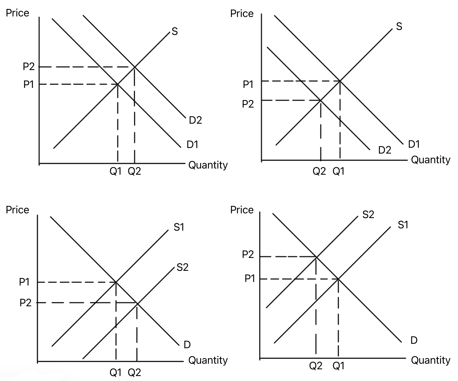
Shifts in Market Equilibrium (Real-World Examples)
Any shift in the demand or supply curve creates a new equilibrium price and quantity.
| Scenario & Cause | Curve Shift | Effect on Equilibrium | Diagram Process |
|---|---|---|---|
|
1. Demand Increase (e.g., product becomes fashionable) |
D curve shifts RIGHT. | P ↑, Q ↑ |
1. D shifts right. 2. At old P1, excess demand exists. 3. Price rises to new equilibrium P2, Q2. |
|
2. Demand Decrease (e.g., fall in real incomes for a normal good) |
D curve shifts LEFT. | P ↓, Q ↓ |
1. D shifts left. 2. At old P1, excess supply exists. 3. Price falls to new equilibrium P2, Q2. |
|
3. Supply Increase (e.g., a government subsidy or new technology) |
S curve shifts RIGHT. | P ↓, Q ↑ |
1. S shifts right. 2. At old P1, excess supply exists. 3. Price falls to new equilibrium P2, Q2. |
|
4. Supply Decrease (e.g., higher raw material costs or a supply shock) |
S curve shifts LEFT. | P ↑, Q ↓ |
1. S shifts left. 2. At old P1, excess demand exists. 3. Price rises to new equilibrium P2, Q2. |
Exam Preparation
- Define and identify market equilibrium on a diagram.
- Analyse situations of excess demand and excess supply, explaining the market forces that return the market to equilibrium.
- Draw clear diagrams to show the impact of changes in demand/supply conditions on equilibrium price and quantity.
- Explain the process step-by-step: (1) State which curve shifts and why. (2) Identify the resulting excess demand/supply at the initial price. (3) Explain how price changes to clear the market. (4) State the final effect on P and Q.
- Apply this analysis to a wide range of real-world contexts (e.g., weather affecting harvests, new regulations, changes in consumer trends).